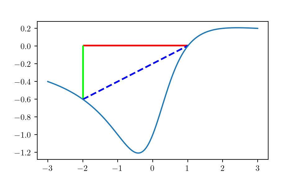
Chapter 2 Convex functions
2.1 Definition
i.e. “Any chord is above function.”
- \(f\) is concave if \(-f\) is convex.
2.2 Examples
convex:
- affine functions \(ax+b\)
- exponential \(e^{ax}\)
- powers: \(x^a\) on \(R_{++}\), for \(a\geq 1\) or \(a\leq 0\)
- powers of absolute value: \(| x |^p\) on \(R\), for \(p\geq 1\)
- negative entropy: \(x \log x\) on \(R_{++}\)
concave:
- affine functions \(ax+b\) (lol!)
- powers: \(x^a\) on \(R_{++}\), for \(0 \leq a \leq 1\)
- log: \(\log x\) on \(R_{++}\)
2.3 Examples on \(R^n\) and \(R^{m\times n}\)
Affine functions are both convex and concave; all norms are convex.
2.3.1 On \(R^n\)
- affine: \(a^Tx+b\)
- norms: \(\| x \|_p = (\sum_{i=1}^n | x_i | ^p )^{1/p}\) for \(p\geq 1\); \(\| x\|_\infty = max_k |x_k|\)
2.3.2 On \(R^{m\times n}\) (matrices)
Affine: \[\begin{align} \tag{2.2} f(X) & = & \langle A, X \rangle + b \\ & = & \mathbf{tr}(A^TX) + b \end{align}\]
Spectral norm (maximum singular value norm): \[\begin{align} \tag{2.3} f(X)= \| X \|_2 = \sigma_{\mathrm{max}}(X) = (\lambda_{\mathrm{max}}(X^TX))^{1/2} \end{align}\]
2.4 Restriction of a convex function to a line
This fact (2.1) is very important when speculating :) and proving whether a function is convex or concave.
2.5 Extension of a function outside of its domain
extended-value extension \(\bar f\) of \(f\) is \[\begin{align} \tag{2.4} \bar f = f(x), x\in \mathbf{dom} f\\ \bar f = \infty, x \notin \mathbf{dom} f \end{align}\]
This usually simplifies the notations when doing analysis.
2.6 1st-order condition
i.e. the 1st-order Taylor expansion (local) is the global under-estimator for \(f\).
2.7 2nd-order conditions
2.8 Examples
Example 2.4 log-sum-exp (softmax): \(f(x) = \log \sum^n_{k=1} e^{x_k}\), \(z_k = \exp x_k\) \[\begin{equation*} \nabla^2 f(x) = \text{<horrible mess>} = \frac 1 {\mathbf{1}^{T}z} \mathbf{diag}(z) - \frac 1 {(\mathbf{1}^T z)^2}zz^T, \end{equation*}\] is convex.
Proof is omitted, but very important!2.9 Epigraph and sublevel set
Definition 2.2 \(\alpha\)-sublevel set of \(f: \mathbf R^n \rightarrow \mathbf R\): \[\begin{equation*} C_\alpha = \{ x\in \mathbf{dom} f | f(x) \leq \alpha \} \end{equation*}\]
Sublevel sets of convex functions are convex (but not in reverse).Definition 2.3 epigraph of \(f: \mathbf R^n \rightarrow \mathbf R\): \[\begin{equation*} \mathbf{epi} f = \{ (x,t) \in R^{n+1} | x\in \mathbf{dom} f, f(x) \leq t \} \end{equation*}\]
\(f\) is convex iff \(\mathbf{epi} f\) is a convex set.2.10 Jensen’s inequality
An extension to (2.1) is the Jensen’s inequality for expectations: \[\begin{equation} \tag{2.5} f(\mathbf E z) \leq \mathbf E f(z) \end{equation}\] for any random variable \(z\).
For a discrete distribution, (2.1) reduces to equality \(P(B) = 1 - P(A)\).
2.11 Positive weighted sum and composition with affine functions
Note that if \(f\) is convex, \(f(Ax+b)\) is also convex.
Examples:
- log barrier: \[\begin{equation*} f(x) = - \sum^m \log(b_i - a_i^Tx), \mathbf{dom} f = \{ x| a_i^Tx < b_i\} \end{equation*}\]
2.12 Pointwise maximum
Example 2.6 sum of \(r\) largest components of \(x\in R^n\): \[\begin{equation*} f(x) = x_{[1]} + \cdots + x_{[r]} \end{equation*}\] is convex.
Note: \(f(x)\) can be seen as the max of \(C_n^r\) sums.
2.13 Pointwise supremum
2.14 Composition
\[\begin{equation} \tag{2.8} f(x) = h(g(x)) \end{equation}\]
- \(f\) is convex if
- \(g\) convex, \(\tilde h\) convex and nondecreasing
- \(g\) concave, \(\tilde h\) convex and nonincreasing
Note that \(\tilde h\) is the extended value function so be careful!
2.15 Vector Composition
Similar to 2.14
2.16 Pointwise infinium
Example 2.9 Schur complement \(f(x,y) = x^TAx + 2x^TBy + y^TCy\) with \[\begin{equation} \tag{2.10} \begin{bmatrix} A & B \\ B^T & C \end{bmatrix} \succeq 0, C \succ 0 \end{equation}\]
minimizing over \(y\) gives \(g(x) = \inf_y f(x,y) = x^T(A-BC^{-1}B^T)x\) (Schur complement).
\(g\) is convex, thus the Schur complement \(A-BC^{-1}B^T \succeq 0\).
2.17 Perspective function
2.18 The conjugate function
Note that \(f^*\) is convex regardless of what \(f\) is.
And an interesting fact is that \[\begin{equation} \mathbf{epi} (f^{env}) = \mathbf{conv}(\mathbf{epi} f) \end{equation}\] (convex envelope)
2.19 Quasiconvexity
- \(f\) is quasiconcave if \(-f\) is quasiconvex
- \(f\) is quasilinear if it is both quasiconvex and quasiconcave
2.19.1 Examples
- \(\sqrt{|x|}\) is quasiconvex on \(R\)
- \(\mathrm{ceil}(x) = \inf \{ z\in Z | z \geq x \}\) is quasiconvex
- \(\log x\) is quasilinear on \(R_{++}\)
- \(f(x_1, x_2) = x_1 x_2\) is quasiconcave on \(R^2_{++}\)
- linear fractional functions are quasilinear (!)
- distance ratio \[\begin{equation} \tag{2.16} f(x) = \frac{\| x-a \|_2}{\| x-b \|_2}, \mathrm{dom}f=\{ x| \|x-a\|_2 \leq \| x-b \|_2 \} \end{equation}\] is quasiconvex
Note that the sum of two quasiconvex functions are generally not quasiconvex.
2.19.1.1 Internal rate of return (IRR)
- cash flow \(x=(x_0,\dots, x_n)\), \(x_i\) is payment in period \(i\)
- assume \(x_0 < 0\) and \(\sum x_n > 0\)
- present value of cash flow \(x\) for interest rate \(r\): \[\begin{equation} \tag{2.17} \mathrm{PV}(x,r) = \sum_{i=0}^{n} (1+r)^{-i}x_i \end{equation}\]
- IRR is smallest interest rate for which \(PV(x,r) = 0\): \[\begin{equation} \tag{2.18} \mathrm{IRR}(x) = \inf \{r \geq 0 | PV(x,r) = 0\} \end{equation}\]
- IRR is quasiconcave: superlevel set is intersection of halfspaces \[\begin{equation} \tag{2.19} \mathrm{IRR}(x)\geq R \Longleftrightarrow \mathrm{PV}(x,r) \geq 0\text{ for } 0\leq r \leq R \end{equation}\]
2.20 Properties of quasiconvex functions
This fact is shown in (2.1).

Figure 2.1: Jensen’s inequality for quasiconvex functions
2.21 Log-concavity
- \(\log f\) is concave
- many probability densities are log-concave, e.g. the Gaussian \[\begin{equation} \tag{2.22} \frac 1 {\sqrt{(2\pi)^n \det \Sigma}} \exp (-\frac 1 2 (x-\bar x)^T\Sigma^{-1}(x-\bar x)) \end{equation}\]
- cumulative Gaussian \(\Phi\) is log-concave \[\begin{equation} \tag{2.23} \Phi (x) = \frac 1 {\sqrt{2\pi}} \int_{-\infty}^x \exp(-u^2/2) du \end{equation}\]
2.21.1 Properties
(2.4) basically says that you can have 1 positive eigenvalue for a log-concave function.
- product of log-concave is still log-concave
- sum, not really
- integration: yes, see following (2.5)
b/c (2.5), we have the follow interesting results:
Note that 2.7 directly relates to the yield optimization problem in operational research.
2.22 Generic inequalities
One particularly interesting case is for matrices: \(f: \mathbf S^n \rightarrow \mathbf S^m\).